Vulkan Compute Shader Particle System

Technical Breakdown

The technical breakdown explains how the particle renderer operates each frame, covering the compute pipeline that updates particle state, the synchronisation required to transition between simulation and rendering, the GPU resources involved and how they are structured, and the implementation that drives the particle behaviour.

So why utilise compute shaders?

Many operations in computer science benefit from parallelism, especially when working with large datasets where each element performs a calculation independently. Although a CPU can run multiple logical threads across several physical cores, its execution model is still fundamentally sequential, which becomes limiting for workloads of this scale. You could distribute work across multiple threads, but if the goal is fast, simple, highly parallel calculations, hardware designed specifically for that purpose becomes the ideal choice.

This is where GPUs come into play. They’re designed for workloads where the same simple operation must be applied across huge numbers of independent elements (which is exactly why they excel at graphics workloads!), making them ideal for particle updates. Compute shaders are the programmable stage of the compute pipeline - a pipeline separate from the graphics pipeline - and they allow you to dispatch work in one, two, or three dimensions. The GPU’s scheduler then distributes that work across its compute units for massively parallel execution. To make use of this properly, we need to understand compute space...

Compute Space

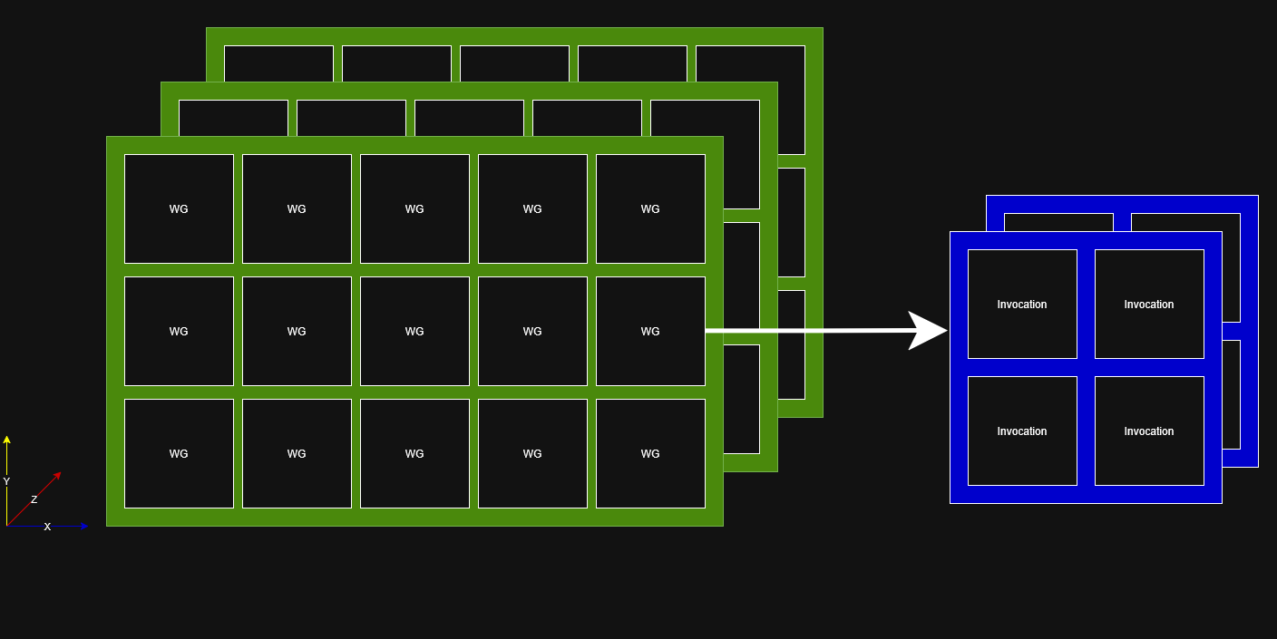
Compute space is an abstraction consisting of 2 fundamentals: "Work Groups" and "invocations". The left‑hand diagram shows the compute dispatch as a stack of 2D slices. Each slice is a layer in Z, and within each layer the dispatch is divided into many workgroups, shown as the small boxes labelled “WG”. The right‑hand diagram is a matching stack of slices for a single workgroup’s local space, where each small box labelled “Invocation” represents one invocation. Together, these two views show how the dispatch is organised into workgroups across 3D space, and how each workgroup in turn contains a grid of invocations.

Within our shader we specify a number of threads – this is our invocation count, and it defines the shape of a single workgroup. When we run the compute shader, we pair that with a dispatch call that tells Vulkan how many workgroups to launch across the entire compute space. The GPU then creates that full 3D grid: every workgroup contains the number of invocations we declared in the shader, and every invocation runs the shader once. This is how the two parts fit together – the shader defines the local structure, the dispatch defines the global structure, and the GPU multiplies them to cover all the data we want to process.

As an example, in the compute shader we specify: [numthreads( 256, 1, 1 )] -this tells the gpu that each workgroup contains 256 invocations arranged along the x dimension. It does not mean that the shader will only run 256 times. You may wonder why we have multiple dimensions for our access patterns. The reason is convenience rather than performance. The GPU doesn’t care whether we dispatch in one, two, or three dimensions - it schedules workgroups as a flat pool i.e it doesn't actually see the dimensions. The dimensionality is for us: it lets our thread IDs match the structure of the data we’re working on. A 2D dispatch is natural when processing textures, and a 3D dispatch fits volumetric data like voxel grids. In our case, we’re working with a simple 1D array of particles, so a 1D workgroup and a 1D dispatch are all we need. If we have 8192 particles and we want 256 threads per workgroup, we would call dispatch(32, 1, 1). This tells the GPU to launch 32 workgroups, each containing 256 invocations. If we chose to dispatch out work across multiple dimensions anyways, it wouldn’t change performance - the GPU schedules workgroups as a flat pool. The dimensionality only affects how we compute our thread IDs, not how fast the work runs.

Invocation size determines how many threads share the same block of workgroup‑local memory. A larger invocation count means more threads synchronising together and more pressure on that shared memory region, but it doesn’t change the size of the memory itself. The hardware limits the maximum number of invocations per workgroup, typically somewhere between 256 and 1024 depending on the GPU. The shader defines the shape of a workgroup. The dispatch defines the quantity of workgroups. The GPU schedules the resulting pool.

With that context explained we can explore the rest of the project!

The particle system

The particle system is relatively simple, each particle has a 2D position, velocity and colour. As this project is to explore the compute shader, we needn't care about realism, the particle just needs to move. Future improvements will be to implement a galaxy simulation where particles orbit a central mass - extending the particles to have mass and gravitational attraction. The particle struct is defined as follows:

                struct particle_t
                {
                   glm::vec2 position;
                   glm::vec2 velocity;
                   glm::vec4 colour;
                   ...
                };
            

Resources

Compute shaders need to arbitrarily read from and write to buffers, vulkan offers shader storage buffer objects (SSBO's) for such a purpose. SSBO's can also hold massive amounts of data, and flexible arrays of variable or dyanamic lengths. SSBO's also support atomic operations, making them suitable for concurrent modifications - exactly how our compute shader works. Here's the declaration for our SSBO in the shader

                struct Particle
                {
                   float2 position;
                   float2 velocity;
                   float4 colour;
                };
                
                struct ParticleSSBO
                {
                   Particle particles;
                };
                
                StructuredBuffer particlesIn;      // Particle state from previous frame
                RWStructuredBuffer particlesOut;   // Particle state to write out for current frame
            

The ParticleSSBO struct is just a container for the particle data, but the important detail is that the shader sees two buffers: a StructuredBuffer for reading and an RWStructuredBuffer for writing. The reason for having both is simple. Each frame, the compute shader needs to read the particle state from the previous frame and write the updated state for the current frame. Reading requires a normal structured buffer. Writing requires a read–write structured buffer. This separation avoids read–write hazards and ensures the simulation always works with stable data.

The compute shader reads last frame’s particle positions and velocities from the StructuredBuffer. It then writes the updated values into the RWStructuredBuffer. On the next frame, these roles swap: the buffer that was written becomes the new read buffer, and the buffer that was read becomes the new write buffer. The buffers themselves never change, but the way they are bound to the shader does. This pattern is known as ping‑pong buffering.

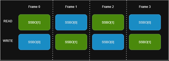
On the application side, this behaviour is implemented by binding two storage buffers in the descriptor set layout:

                        { .binding = 1,
                        .descriptorType = vk::DescriptorType::eStorageBuffer,
                        .descriptorCount = 1,
                        .stageFlags = vk::ShaderStageFlagBits::eCompute },
                        
                        { .binding = 2,
                        .descriptorType = vk::DescriptorType::eStorageBuffer,
                        .descriptorCount = 1,
                        .stageFlags = vk::ShaderStageFlagBits::eCompute }
            

When creating the descriptor sets, one set is created per frame in flight. For each frame, the descriptor set binds two storage buffers: one representing the previous frame’s particle data and one representing the current frame’s output. The modulo operation is used to wrap the index so that frame 0 reads from the last buffer in the array, frame 1 reads from buffer 0, and so on. This is what creates the ping‑pong effect.

                        for (size_t frame_index = 0; frame_index < max_frames_in_flight; frame_index++)
                        {
                        vk::DescriptorBufferInfo storage_buffer_info_last_frame{
                        shader_storage_buffers.at((frame_index - 1) % max_frames_in_flight),
                        0,
                        sizeof(particle_t) * particle_count };
                        
                        vk::DescriptorBufferInfo storage_buffer_info_current_frame{
                        shader_storage_buffers.at(frame_index),
                        0,
                        sizeof(particle_t) * particle_count };
                        
                        // Write both bindings into the descriptor set
                        vk::WriteDescriptorSet{
                        .dstSet = *compute_descriptor_sets.at(frame_index),
                        .descriptorType = vk::DescriptorType::eStorageBuffer,
                        .pBufferInfo = &storage_buffer_info_last_frame,
                        ... };
                        
                        vk::WriteDescriptorSet{
                        .dstSet = *compute_descriptor_sets.at(frame_index),
                        .descriptorType = vk::DescriptorType::eStorageBuffer,
                        .pBufferInfo = &storage_buffer_info_current_frame,
                        ... };
                        }

Binding one buffer as “last frame” and one as “current frame” ensures the compute shader always reads stable data and writes new data without conflicts. The descriptor layout determines which buffer appears as StructuredBuffer and which appears as RWStructuredBuffer inside the shader. The buffers themselves remain fixed; only their roles change from frame to frame.

The compute shader

Each frame we bind the compute pipeline and dispatch our compute work. The compMain function looks as follows. (based on Sascha Willems' vulkan compute example)

        [shader( "compute" )]
        [numthreads( 256, 1, 1 )]
        void compMain( uint3 threadId: SV_DispatchThreadID )
        {
           // Firstly set position
           uint index = threadId.x;
           particlesOut[index].particles.position =
              particlesIn[index].particles.position + particlesIn[index].particles.velocity.xy * ubo.delta_time;
        
           // Set velocity
           particlesOut[index].particles.velocity = particlesIn[index].particles.velocity;
        
           // Flip the movement when we hit the window border
           if (
              ( particlesOut[index].particles.position.x <= -1.0 ) ||
              ( particlesOut[index].particles.position.x >= 1.0 ))   // Flip x
           {
              particlesOut[index].particles.velocity.x = -particlesOut[index].particles.velocity.x;
           }
           if (
              ( particlesOut[index].particles.position.y <= -1.0 ) ||
              ( particlesOut[index].particles.position.y >= 1.0 ))   // Flip y
           {
              particlesOut[index].particles.velocity.y = -particlesOut[index].particles.velocity.y;
           }
        }

As described before, the numthreads we specify here uses 256 threads in the x dimension. Each thread is indexed using "index" which corresponds to the thread ID. We use it to index our particles from the input buffer. The compute shader is relatively simple, it reads the particle position and velocity from the input buffer, updates the position based on the velocity and delta time, and then checks if the particle has hit the window border. If it has, it flips the velocity in that direction. The updated position and velocity are then written to the output buffer. This process is repeated forevery particle in parallel, allowing for efficient simulation of large numbers of particles.

Synchronisation

Synchronisation is one of Vulkan’s core concepts, and it’s essential for ensuring that the compute shader runs correctly and that the data it reads and writes is properly ordered. In this project, synchronisation happens at two levels. First, we need to ensure correct ordering between command buffer submissions, so that the compute pass for a frame finishes before the graphics pipeline reads the updated particle data. For this a timeline semaphore is used.

                
            ...
            // update timeline value for frame
              uint64_t compute_wait_value = timeline_value;
              uint64_t compute_signal_value = ++timeline_value;
              uint64_t graphics_wait_value = compute_signal_value;
              uint64_t graphics_signal_value = ++timeline_value;   
              {
                 vk::TimelineSemaphoreSubmitInfo compute_timeline_info{
                    .waitSemaphoreValueCount = 1,
                    .pWaitSemaphoreValues = &compute_wait_value,
                    .signalSemaphoreValueCount = 1,
                    .pSignalSemaphoreValues = &compute_signal_value };
                
                 vk::PipelineStageFlags wait_stages = { vk::PipelineStageFlagBits::eComputeShader };
                
                 vk::SubmitInfo compute_submit_info{
                    .pNext = &compute_timeline_info,
                    .waitSemaphoreCount = 1,
                    .pWaitSemaphores = &*semaphore,
                    .pWaitDstStageMask = &wait_stages,
                    ...
                    .signalSemaphoreCount = 1,
                    .pSignalSemaphores = &*semaphore };
                
                 queue.submit( compute_submit_info, nullptr );
              }

One thing I’ve learned is that Vulkan synchronisation only makes sense when you stop treating it as a procedural sequence and start thinking of it as a set of ordering relationships. The timeline semaphore values in this project encode those relationships. Each frame’s compute submission waits on the value that represents the previous frame’s work, because that work must have completed before the new compute pass can safely read from the storage buffer. Once the compute pass finishes, it signals the next value, advancing the timeline.

The graphics submission uses that newly signalled value as its wait point. This ensures that the graphics pipeline only reads from the storage buffer after the compute shader has finished writing to it. The graphics submission then signals its own value, which becomes the wait point for the present queue. In effect, each stage waits on the stage before it and signals the stage after it. The timeline values simply express that ordering.

Since buffers in vulkan have multiple uses, we are able to use our shader storage buffer for drawing. When we come to draw our particles we use the following:

command_buffer.bindVertexBuffers( 0, { shader_storage_buffers.at( frame_index ) }, { 0 } );

What I learned

In this project I learned how compute space works in practice and how to correctly implement a compute shader in Vulkan. I built a clearer understanding of how compute workloads are dispatched, how buffer storage types behave, and what constraints they impose on shader design. I also deepened my knowledge of synchronisation, particularly around timeline semaphores, and gained confidence in structuring correct ordering between compute and graphics submissions. This was important because the tutorial I originally followed relied on implicit synchronisation, and I wanted to ensure that my own implementation handled ordering explicitly and correctly. Overall, this project strengthened my understanding of Vulkan’s model and gave me a solid foundation for more advanced GPU simulation work. In the future, I’d like to extend this into a galaxy simulation or explore 3D rigid body interactions using a voxel grid.